Welcome to the first in a series of posts on magnetic moments. In this post where we’re going to look at the Stern-Gerlach experiment from a classical perspective.
It was discovered experimentally, in 1922 by Stern and Gerlach (SG), that the spin of an electron along any direction is quantised, taking values of either \(\hbar/2\) or \(-\hbar/2\). The experiment involved firing silver atoms into an inhomogeneous magnetic field and observing a splitting of the beam in the direction of the field inhomogeneity.
Since then, people have described an idealised system of many SG systems in parallel that are capable of splitting apart and recombining the particle beams together (often called a Stern-Gerlach interferometer) to create interference effects that are commonly discussed in the two slit experiment (see e.g. the Feynman lectures).
To my surprise, it is only very recently that Stern-Gerlach interferometer experiments are being considered practical enough to implement and yet they are used frequently as a pedagogical example. It is therefore worth first developing an intuition for what one might expect from such SG interferometer experiments using only classical physics. That is the purpose of this post.
This post has been created directly from a Jupyter notebook that’s hosted in the magnetic-moments Github repo. That notebook simulates classical particles moving through an idealised SG apparatus. You can therefore expect to see blocks of code, results of code execution and my commentary throughout this post.
Libraries
1# need this to use the cross product later
2using LinearAlgebra
3
4# using Plots http://docs.juliaplots.org/latest/install/
5# https://gist.github.com/gizmaa/7214002 - examples uing PyPlot in Julia
6using PyPlot
Physical constants
 1# The g-factor https://en.wikipedia.org/wiki/G-factor_(physics)
 2g=2
 3
 4# Bohn magneton
 5mu_B = 9.27400968e-24;
 6
 7# electron charge
 8e = 1.602176634e-19
 9
10# electron mass (not needed but I have it here in case I need it later)
11m_e = 9.1093837015e-31
12
13# magnetic moment of the electron (ignoring g-factor corrections for now, i.e. g=2)
14mu_e =  mu_B
15
16# mass of silver atom
17m_Ag = 107.9*1.66053906660e-27
18
19# gyromagnetic ratio https://en.wikipedia.org/wiki/Gyromagnetic_ratio
20gyro =  g*e/(2.0*m_Ag)
21
22# magnetic moment of silver (same as a single electron because Ag has 1 electron in outer shell)
23mu_Ag =  mu_e
24
25# speed of light
26c = 299792458;
Experimental set-up
A 2009 paper by França on “The Stern–Gerlach Phenomenon According to Classical Electrodynamics” describes a lot of the set-up and parameters, e.g.
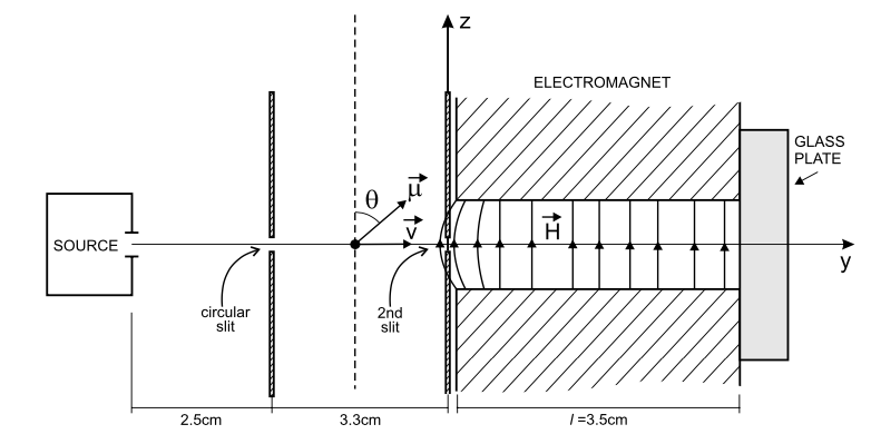
An approximation for the magnetic field inside the electromagnet (length 3.5cm) is described by França’s Eq 23:
\[ B = (-\beta x, 0, B_0 + \beta z) \]
with \( \beta = 1800\) explicitly stated at the bottom of page 1186 and \(B_0\) inferred from França’s Fig 3 and checked in Fig. 5 of Rabi’s original paper.
1# max B field inside the electromagnet
2B0 = 1.4
3
4# x and z B field gradient inside the electromagnet
5beta = 1800
6
7# electromagnet dimesion in y
8# note, I cannot find dimensions for x and z
9machine_dim_y = 0.035;
To start with, we’ll simulate a particle moving through the electromagnet only and deal with what happens at the magnet entrance later on.
Let’s explore the B field given França’s parameters.
1function B(r)
2    B = zeros(3)
3    B[1] = -beta*r[1]
4    B[3] = B0 + beta*r[3]
5    return B
6end;
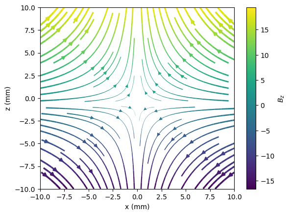
We can visualise the B field lines and also the strength of B in the x,z plane:
1r = [[j,0,i] for i=-0.01:0.0001:0.01, j=-0.01:0.0001:0.01];
2x = [x for (x,y,z) in r]
3z = [z for (x,y,z) in r];
1B_calc = B.(r)
2B_calc_x = [Bx for (Bx,By,Bz) in B_calc]
3B_calc_z = [Bz for (Bx,By,Bz) in B_calc]
4B_norm = norm.(B.(r));
1st = streamplot(x*1000, z*1000 ,B_calc_x, B_calc_z, linewidth=3*Bnorm/maximum(Bnorm), color=B_calc_z)
2cb=colorbar(st.lines)
3cb.set_label(L"B_z")
4xlabel("x (mm)")
5ylabel("z (mm)");
1con = contour(x.*1000, z.*1000, B_norm, levels=20)
2xlabel("x (mm)")
3ylabel("z (mm)")
4clabel(con, inline=1, fontsize=10);
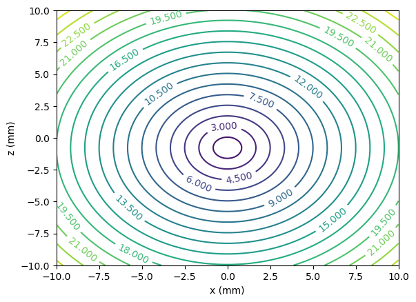
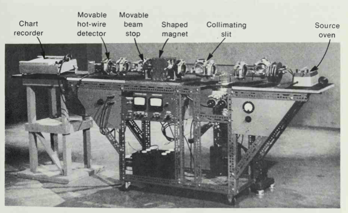
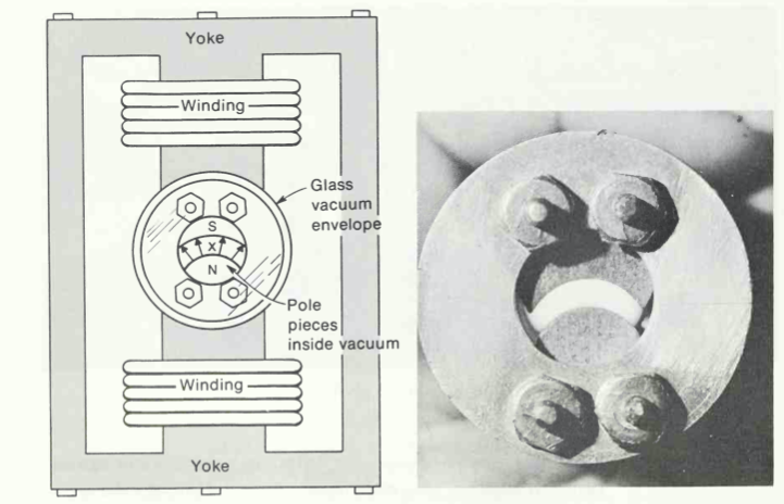
This field is very strong! To get a sense of what equipment generates these fields, below are figures taken from the book An Introduction to Quantum Physics by French. This book is referenced in the França paper as a “modern” SG experiment.
Equations of motion for a magnetic moment in a B field
If we consider an infinitesimal current loop, then the magnetic moment \(\mu\) is:
\[ \mu = IA \]
where \(I\) is the current of the loop and \(A\) is its area. The force on the loop is:
\[ \nabla(\mu\cdot B) \]
and the torque is:
\[ \tau = \mu \times B \]
cf. wikipedia.
Recalling that:
- a current loop has angular momentum \(L=\mu/\gamma\) where \(\gamma\) is the gyromagnetic ratio
- the magnetic moment is not a function of position
we can write some equations of motion:
\[ \frac{dv}{dt} = \frac{1}{m} \mu \nabla B \]
\[ \frac{d\mu}{dt} = \gamma \mu\times B \]
where \(\nabla B\) is the gradient of the vector B (i.e. a tensor) with components \(\nabla B_{ij} = \partial B_i / \partial x _i\) which we can calculate using the function below.
1function gradB(r)
2    gradB = zeros(3,3)
3    gradB[3,3] = beta
4    gradB[1,1] = -beta
5    return gradB
6end;
From the equations of motion above we can expect:
- the magnetic moment to move in the direction of gradients in the field
- the orientation of the magnetic moment will precess about the direction of the magnetic field (see Larmor precession)
Set-up initial values for the simulation
We’ll start the particles off with velocity only in the y direction at \(v_0 = 600 \ m/s\) (see end of page 1181 of França article).
We’ll initialise a random orientation of the magnetic moment using a spherical coordinate system:
\[ \mu = [\sin(\theta)\cos(\phi), \ \sin(\theta)\sin(\phi), \ \cos(\theta)]\mu_{Ag} \]
where \(\theta\) and \(\phi\) are the spherical angle coordiantes corresponding to the ISO convention. In order to ensure a uniform distribution we must choose
\[ \theta = \arccos(2\times rand()-1) \]
\[ \phi = 2\pi\times rand() \]
as dicussed here.
Because we expect some precessional motion, we should choose a time-step that resolves it. The Larmor frequency \(\omega = \gamma B\) is a good guide for this. We therefore need a timestep \(\Delta t < 2\pi/\omega\):
12*pi/(gyro * B0)
5.018939737048401e-6
 1v0 = 600.0
 2v = [0,v0,0]
 3r = [0,0,0]
 4
 5theta = acos(2*rand()-1)
 6phi = rand()*2*pi
 7mu = [sin(theta)*cos(phi), sin(theta)*sin(phi), cos(theta)]*mu_Ag
 8
 9dt = 1.0e-7
10t_max = machine_dim_y/v0
11times = collect(0:dt:t_max)
12
13
14r_save = zeros(length(times),3)
15mu_save = zeros(length(times),3);
Solving the equations of motion
To numerically solve equations of motion:
\[ \frac{dv}{dt} = \frac{1}{m} \mu \nabla B \]
\[ \frac{d\mu}{dt} = \gamma \mu\times B \]
we employ an algorithm that’s a hybrid of leapfrog and the Boris method.
 1function frog_boris(r,v,mu)
 2
 3    # leapfrog kick
 4    v += (0.5*dt*(mu'*gradB(r))/m_Ag)'
 5
 6    # Boris
 7    Br = B(r)
 8    s = 2.0/(1+(norm(Br)*gyro*dt*0.5)^2)
 9    mu_prime = mu + 0.5*dt*gyro*cross(mu,Br)
10    mu += 0.5*dt*gyro*s*cross(mu_prime,Br)
11
12    # leapfrog drift
13    r += dt*v
14
15    # leapfrog kick
16    v += (0.5*dt*(mu'*gradB(r))/m_Ag)'
17
18    return r, v, mu
19end;
1for (i,t) in enumerate(times)
2
3    r_save[i,:] = r
4    mu_save[i,:] = mu
5
6    r, v, mu = frog_boris(r, v, mu)
7
8end
Visualise the single particle results
 1# In case we simulate lots of points and we don't want to plot them all because of memory,
 2# we can plot every 'n' points
 3n = 1
 4times_plot = times[1:n:end]./1e-6
 5r_save_plot = r_save[1:n:end,:]./1e-3
 6mu_save_plot = mu_save[1:n:end,:]./mu_B;
 7mu_norm_plot = [norm(mu_save_plot[i,:]) for i=1:size(mu_save_plot,1)]
 8
 9figure(figsize=(8,10))
10
11subplot(411)
12plot(times_plot,(r_save_plot[:,3]), label="z");
13ylabel("z (mm)")
14
15subplot(412)
16plot(times_plot,(r_save_plot[:,2]), label="y");
17ylabel("y (mm)")
18
19subplot(413)
20plot(times_plot,(r_save_plot[:,1]), label="x");
21ylabel("x (mm)")
22
23subplot(414)
24plot(times_plot,mu_save_plot[:,1], label=L"$\mu_x$")
25plot(times_plot,mu_save_plot[:,2], label=L"$\mu_y$")
26plot(times_plot,mu_save_plot[:,3], label=L"$\mu_z$")
27plot(times_plot,mu_norm_plot, label=L"$\mu$")
28xlabel(L"time ($\mu$s)")
29ylabel(L"magnetic moment ($\mu_B$)")
30legend(loc="right");
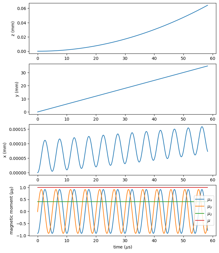
Because we initialised the magnetic moment at \(x=0\), where \(B_x=0\), the precession started around the z direction and so we see an oscillation of the \(\mu_x\) and \(\mu_y\). Because the \(\mu_x\) oscillates, the force from the gradient of B in x also oscillates which creates the ripple in the x position.
Simulating many particles
There are many things we can change about the initial conditions when simulating many particles, we can create a distribution of positions, of speeds, of magnetic moments etc. Let’s begin with creating a distribution of magnetic moments. This simply means running the code above many times, picking a different random \(\mu\) every time.
Because most of the interest in the SG experiment is in the final z distribution of the particles after they have gone through the magnet, we’ll store the final z position and visualise how they are distributed.
 1# number of particles
 2np = 1000
 3
 4# place to store the final z-position
 5zs = zeros(np)
 6
 7for p in 1:np
 8
 9    v = [0,v0,0]
10    r = [0,0,0]
11    theta = acos(2*rand()-1)
12    phi = rand()*2*pi
13    mu = [sin(theta)*cos(phi), sin(theta)*sin(phi), cos(theta)]*mu_Ag
14
15
16    for (i,t) in enumerate(times)
17
18        r,v,mu = frog_boris(r,v,mu)
19
20    end
21
22    zs[p] = r[3]
23
24end
1hist(zs/1e-3, normed=true);
2xlabel("z (mm)");
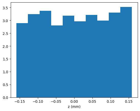
We can see that there is a pretty even distribution of z’s as one might expect - nothing controversial.
Including edge effects
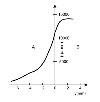
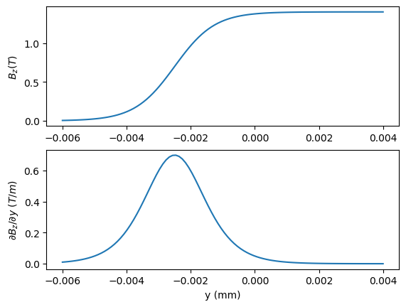
The França paper makes the case that the SG results can be explained classically as being caused by the inhomogeneity in the magnetic field along y. Specifically, the magnetic field goes from being zero outside the magnet to a maximum inside the magnet over a very short length scale (cf Fig 3 of França):
França shows that if the energy of the particle and electromagnet are considered together, then the work done by (or on) the magnet, as the particle enters, leads to a change of \(\theta\) (the angle of \(\mu\) with respect to z axis) according to:
\[ \dot \theta = - \frac{v_y}{B_z(y)}\frac{\partial B_z(y)}{\partial y} \cot(y) \]
One can begin to think about trying to verify this through simulation by first creating some approximations for the edge field, e.g.
 1z = LinRange(-0.006,0.004,100)
 2
 3subplot(211)
 4B_edge = B0.*(0.5.*tanh.(800.0.*z.+2.0).+0.5)
 5plot(z,B_edge)
 6ylabel(L"B_z (T)");
 7
 8subplot(212)
 9B_edge_grad = B0.*0.5.*sech.(800.0.*z.+2.0).^2
10plot(z,B_edge_grad)
11xlabel("y (mm)");
12ylabel(L"\partial B_z /\partial y \ (T/m)");
We can re-create the field and gradient functions to include the new inhomogeneity.
1function B(r)
2    B = zeros(3)
3    B[1] = -beta*r[1]
4    B[3] = B0.*(0.5.*tanh.(800.0.*r[3].+2.0).+0.5);
5    return B
6end;
1function gradB(r)
2    gradB = zeros(3,3)
3    gradB[3,3] = beta
4    gradB[1,1] = -beta
5    gradB[3,2] = B0.*0.5.*sech.(800.0.*r[3].+2.0).^2
6    return gradB
7end;
and then re-run the simulation code for many particles:
 1# number of particles
 2np = 1000
 3
 4# place to store the final z-position
 5zs = zeros(np)
 6
 7for p in 1:np
 8
 9    v = [0,v0,0]
10    r = [0,0,0]
11    theta = acos(2*rand()-1)
12    phi = rand()*2*pi
13    mu = [sin(theta)*cos(phi), sin(theta)*sin(phi), cos(theta)]*mu_Ag
14
15
16    for (i,t) in enumerate(times)
17
18        r,v,mu = frog_boris(r,v,mu)
19
20    end
21
22    zs[p] = r[3]
23
24end
1hist(zs/1e-3, normed=true);
2xlabel("z (mm)");
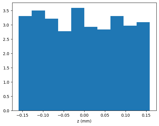
There is again nothing striking in the above figure, the distribution is again pretty uniform. We might wonder whether we have sufficient resolution of the inhomogeneity, if not then maybe that’s why we don’t see any difference. Let’s see:
1# time to traverse the Bz ramp
2ramp_time = 4e-3 / v0
6.666666666666667e-6
1# how many time steps do we have while the particle is in the Bx ramp
2ramp_time/dt
66.66666666666667
We seem to have enough resolution, so that’s not the problem.
Perhaps the problem lies in our current equations of motion: \[ \frac{dv}{dt} = \frac{1}{m} \mu \nabla B \]
\[ \frac{d\mu}{dt} = \gamma \mu\times B \]
There does not appear to be an obvious way that the inhomogeneity in the field can affect \(\mu\) in the way described by França. Our equations are however not complete - there are several non-quantum options for modifying the equations of motion to include more physics. We could:
- Include self consistent equations for the magnetic field - this would be in the spirit of the França paper.
- Go beyond the infinitesimal magnetic dipole approximation, i.e. beyond \(\tau = \mu \times B\). Rather than considering only the dipole contributions to the torque perhaps we could also look at the quadrupole terms.
- Add in relativistic effects arising from the accelerating motion of the particle, so called Thomas precession.
We’ll consider relativity first.
Thomas precession
In addition to the Larmor precession of \(\mu\) that we’ve described in our equations of motion, there is another term called Thomas precession. This precession arises from the acceleration of the particle (whose magnetic movement we are trying to describe). When the particle accelerates, its instantaneous rest frame turns out to rotate with angular velocity \(\omega\) given approximately (for non-relativistic speeds) by: \[ \omega \approx \frac{1}{2c^2}a\times v \] where \(a\) is the acceleration and \(v\) the velocity.
In rotating frames, the equations of motion need to be modified because the corodinate system itself is time-dependent. Working through the details, one finds: \[ \frac{d}{dt}_{rot} = \frac{d}{dt}_{rest} + \omega \times \] The equation of motion for \(\mu\) therefore needs to be modified to give: \[ \frac{d \mu}{dt} = \gamma\mu \times B +\frac{1}{2c^2}(a\times v)\times \mu \] Substituting the particle acceleration \(\frac{dv}{dt} = \frac{1}{m} \mu \nabla B\), we get: \[ \frac{d \mu}{dt} = \gamma \mu \times \left[ B -\frac{1}{2\gamma mc^2}(\mu\nabla B)\times v \right] \]
The Thomas precession creates an effective additional magnetic field of size \(\frac{1}{2\gamma mc^2}(\mu\nabla B)\times v\). It is of course interesting to consider the consequences of such an effective field, but we can immediately get a sense of the importance of this effective field by plugging in some characteristic numbers from the SG experiment.
1Thomas_effective_field = mu_Ag*beta*v0/(gyro*m_Ag*c^2) # recall that beta is the gradiant of the magnetic field
2Thomas_effective_field
6.955678509487803e-16
Compare this to the real magnetic field:
1B0
1.4
The Thomas precession of the magnetic moment is 16 orders of magnitude smaller than the Larmor precession. It’s therefore difficult to imagine that it will have much part to play in understanding the results of the SG experiment. In addition, a modification of the precession alone doesn’t appear to provide the right kind of physics to bias \(\mu_z\) away from zero (which is what’s França is claiming is possible using classical physics).
To be continued